 The famous selfie shared by Ellen DeGeneres with actors, front row from left, Jared Leto, Jennifer Lawrence, Meryl Streep, Ellen DeGeneres, Bradley Cooper, Peter Nyongo Jr. and, second row, from left, Channing Tatum, Julia Roberts, Kevin Spacey, Brad Pitt, Lupita Nyongo and Angelina Jolie during the Oscars 2014 (AP Photo/Ellen DeGeneres) (AP)
“It’s Not What You Know. It’s Who You Know”
Everyone has heard this quote or experienced it firsthand. It is no secret that social networks greatly impact career and personal life.
This claim also holds true in the movie industry, and maybe more than others. In this project, we analyzed the social network of people who work in the movie industry. We used the CMU Movie Summary Corpus and IMDb datasets to do our analysis.
We analyzed the large social network by dividing it into clusters and then zoomed into the significant clusters to investigate further why these clusters exist and who are the key people that bridge different clusters. We looked at each cluster’s common attributes and tied them into real movie industries.
Our research questions,
- Are there clusterings between the people in the film industry?
- What are the common attributes of people in the same cluster?
- Are there people without a cluster? What makes them unique?
- As representation and diversity have more space in conversations today, do we observe the same awareness in the film industry?
- Are women employed equally to men?
- How diverse is each cluster?
The Data We Worked With
We merged IMDb dataset into our given dataset to have more entries and features such as ethnicity which we will use in the later stages. Since we are investigating the connections between people, we wanted to minimize the matches between people who would not be able to meet in real life due to the year they were active. To choose the best period, we looked at the number of movies per year.
As seen from the plot, the 1996-2011 (both inclusive) period has the highest number of movies. We have 14800 movies, and 74973 people with 38 different professions. One may ask why didn’t we just count the number of people and select a period. The answer will be clear after understanding what we are trying to visualize with the dataset.
How to visualize?
First and foremost, we are interested in how people are connected. Building a network graph is the best way to illustrate this. Thus, we need to define the nodes and edges of the graph. Nodes represent people, and an undirected edge between two people exists if they worked in the same movie. To make our network less sparse, we made our initial period decision on movie count. Intuitively, when two people work with each other more, they build a stronger connection. To represent this, our edges are weighted by common number of movies.
Now, let’s build our graph to visualize what we talked about.
We turned our attention to the Fruchterman-Reingold force-directed algorithm, which produces beautiful networks. Those graphs emphasize the position of the nodes, assuring as few edge crossings and distance disparities as possible. The algorithm works similarly to the interaction between attractive and repelling forces. The edges between nodes are the springs that pull closer, and the nodes themselves are the object exerting push.
🔎 Use the built-in magnifying glass to take a closer look.
📥 To download the full resolution image, click here.

Clustering
We see some natural clusterings, so we run a clustering algorithm to understand why. We used OPTICS clustering algorithm, which has foundations from DBSCAN but allows rejecting clusters under a specific size. We rejected clusters under 400 people to focus on more generalizable clusters.
To simplify the graph, we only show the names of people who were in more than 24 movies.
🔎 Use the built-in magnifying glass to take a closer look.
📥 To download the full resolution image, click here.

Looking at the cluster graph, we observe five large clusters (differentiated by color) and some outliers. We are curious whether these clusters represent or resemble real clusters such as Hollywood, Bollywood, etc. The name of these movie industries comes from where they are located. For example, Hollywood is a neighborhood in Los Angeles, California, USA and Bollywood gets its name from its birthplace, Bombay (now Mumbai), India. Since movies generally cater to the local audience, native languages are used. This also means that the majority of the actors, directors and writers are from that nationality or native speakers of the language.
From this analogy, we can use the ethnicity to reveal which movie industry the clusters resemble. The ethnicity information comes from the CMU dataset and is available only for actors. But we can assume that the distribution of the people with ethnicities (although a small percentage) will be in line with the distribution if all entries had the feature.
Diving into clusters
Let’s plot the ethnicity distribution of each cluster. We only considered non-NaN values for the plotting and the plots show the five most occured ethnicities in each cluster. Note that the results of the clusters heavily depend on the algorithm and the parameters we used.

Cluster 1: We can see that Americans with different descents are observed the most, with ~34%. Thus we can say that this is the cluster that represents Hollywood.
Cluster 2: This cluster represents Bollywood, with 60% Indian population. Punjabis who live in eastern Pakistan and northwestern India are also considered active in Bollywood cinema. We will call this cluster Bollywood (North).
Cluster 3: This cluster is rather interesting. It has an equal percentage of Japanese and Chinese Americans. Then we have two more ethnicities of Asian descent. So we can call this Asian Cinema.
Cluster 4: This one is Korean Cinema with more than 80% Koreans in it.
Cluster 5: We also see Indians as a majority ethnicity similar to Cluster 2. The difference is the second biggest ethnicity, the Tamils are from India (Southern regions) and Sri Lanka. So this is also Bollywood; to distinguish, we will call this Bollywood (South).
Let’s plot the ethnicity plot again with new cluster names; we will use these names for each cluster from now on.
Since we named the clusters, we can look further into some interesting statistics.
Popular Genres
Depending on many factors such as culture and history, each audience enjoys different movie genres. We decided to plot the genre distribution of the IMDb dataset because CMU genres are more specific but less consistent due to the crowdsourcing nature of data. And IMDb genres are fewer (19 of them) but more consistent.
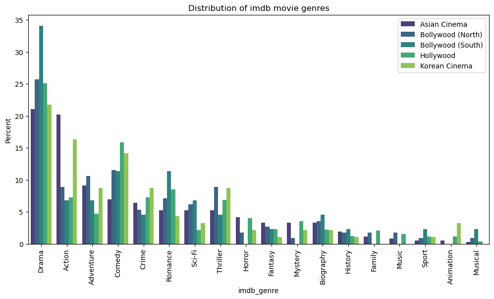
Drama is a favorite of all clusters. It is by far the most popular genre in Bollywood, whereas in Asian cinema Action movies are as popular as drama movies. Comedy comes second in Hollywood. In Korean Cinema, we see a more equal distribution between genres.
Globally, drama movies made around $42 billion in the 90s and $75 billion in the 2000s. Adventure and action movies made around $26 billion and $29 billion, respectively, during the 90s and by the end of 2010. (Source: Box Office Mojo)
Profession
Our dataset has people with different professions such as actor, actresses, editors, etc. Let’s take a look.
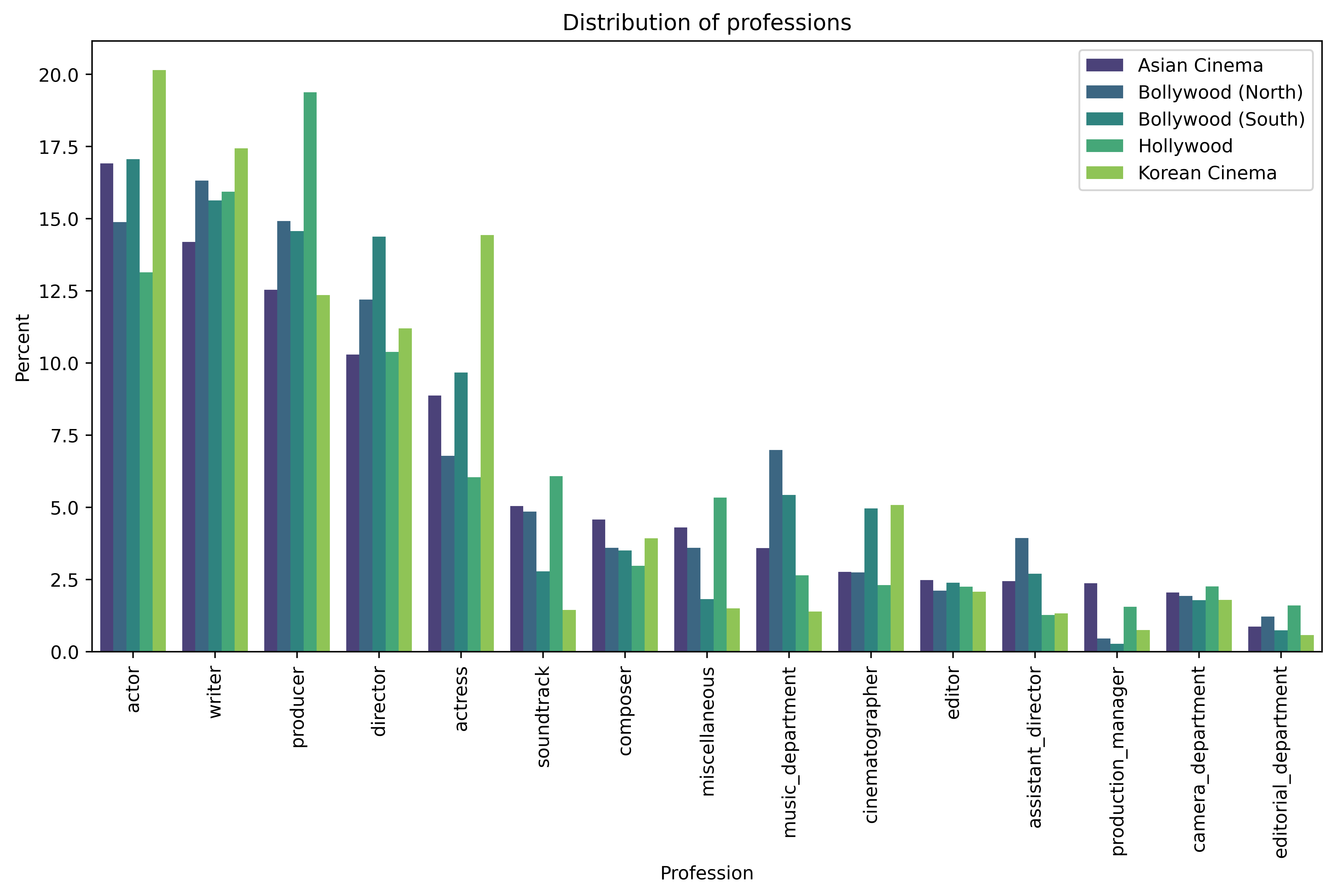
The professions data comes from IMDb, and is generated from the credits. If we focus on the professions with a higher percentage, they being actors, actresses, producers and directors, we see that all clusters have similar distribution with 5-10% difference.
Interestingly, we have much more actors than actresses with a significant difference. According to New York Film Academy, there are 2.25 actors for one actress. Does this inequality happen also behind the scenes? Let’s look at the general gender percentage.
Gender
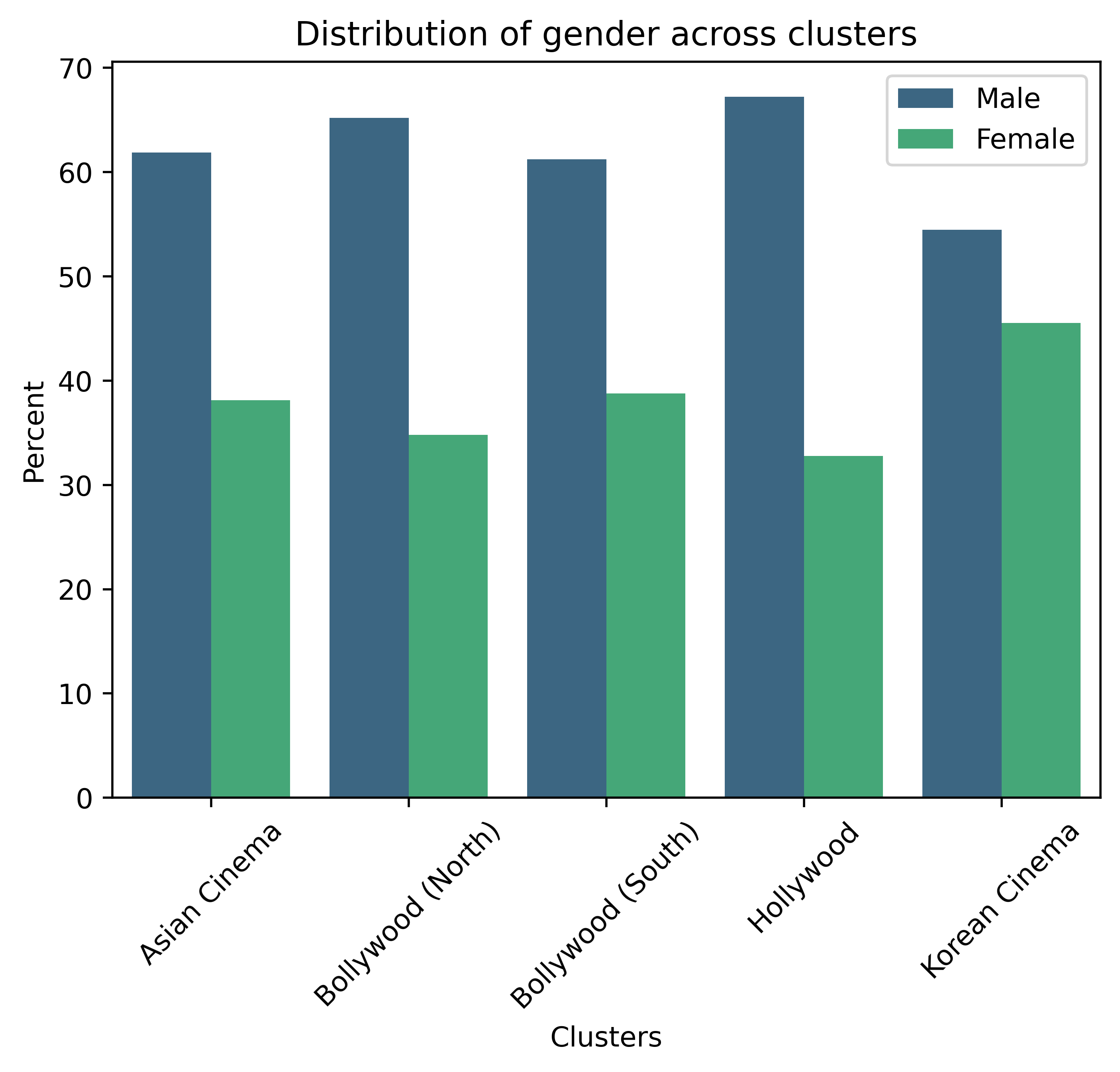
Unfortunately, we see a deeper cut between male and female employment. Korean Cinema seems to be the most inclusive with only a 10% difference. Hollwood has almost 30% difference, meaning there is one female per two males. And this is very recent times! 75.25% of people in our dataset have a gender attribute, so these results truly reflect the actual distribution.
Globally, the ratio of men working in the movie industry to women is 5:1. (Source: New York Film Academy)
Age
In movies, we often see characters of different ages, which means an actor/actress can do their profession for a long time. But with any performative job, they have their “golden years”. We are curious to see what these golden years mean for each cluster. We calculated the age of actors and actresses by taking the difference between the year the movie was released and their birthdays. Note that since some people played in multiple movies during the evaluation period, they are counted more than once. We removed Bollywood (South) cluster in our analysis since we only had two people who with a valid age value.
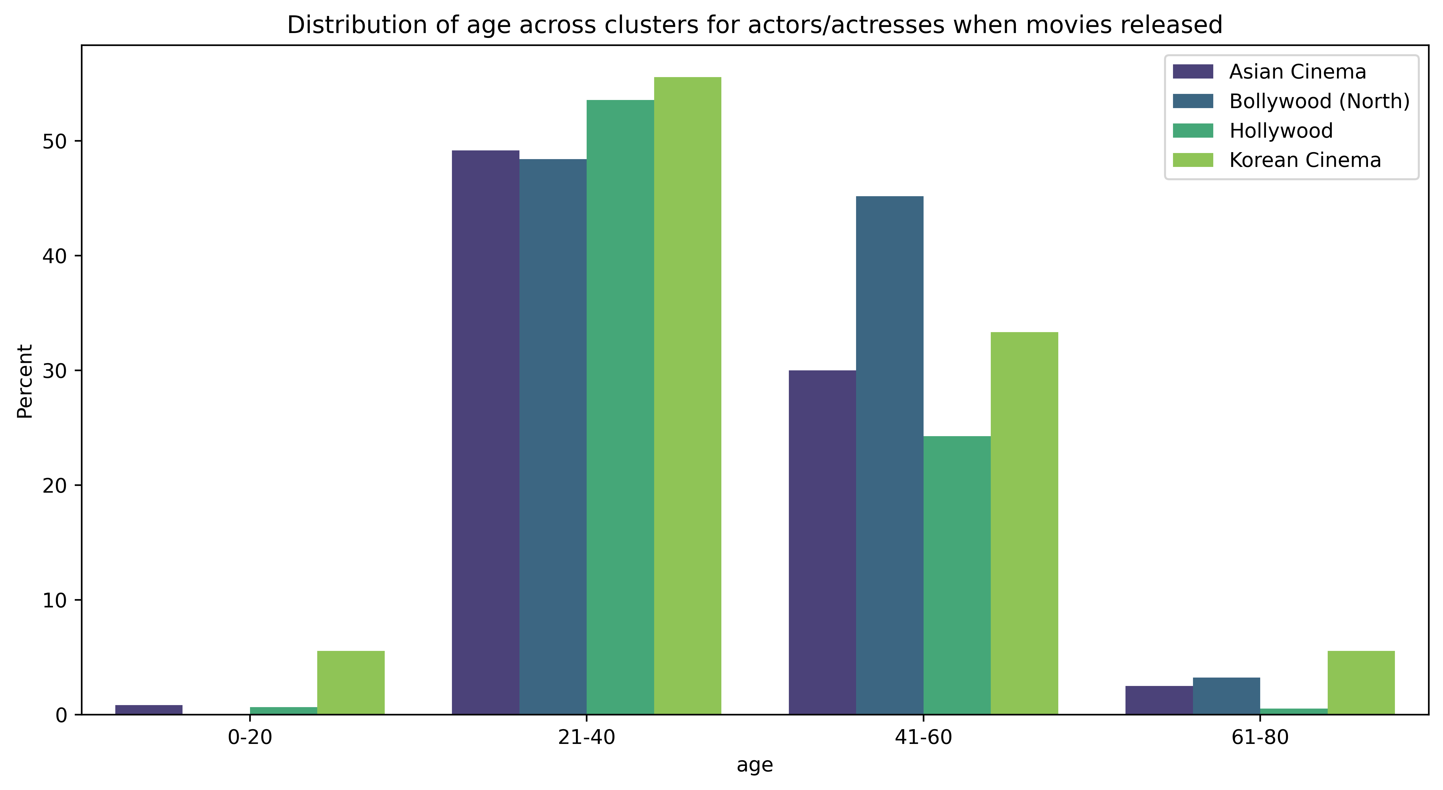
Not to our surprise, 21-40 years old actors and actresses are the majority in all clusters. It is followed by 41-60. We could say that ageism is very clearly seen in Hollywood and Bollywood. Korean Cinema has more representation of young(20-) and old(60+) people.
A recent calculation cited by the Guardian claimed that in 2014’s 20 highest-grossing films, on average, 3 out of 10 actors were women, and only 8% of those actors were between 40 and 59, with a shockingly low 2% over 60. (Source: Reader’s Digest UK)
Outside of the Clusters
Outliers
Before looking at key people, let’s look at outliers. As we saw in the clustering part, we have discovered five clusters in our network, and in addition, more than half (53.4%) of our nodes are outliers. We define outliers as people who are not placed in a cluster. They could be marked as due to working with people from different clusters; we will look into this.
Despite us classifying them as “outliers”, these people are of course still connected to the other people. Let us compare the connectivity between each cluster and outliers.
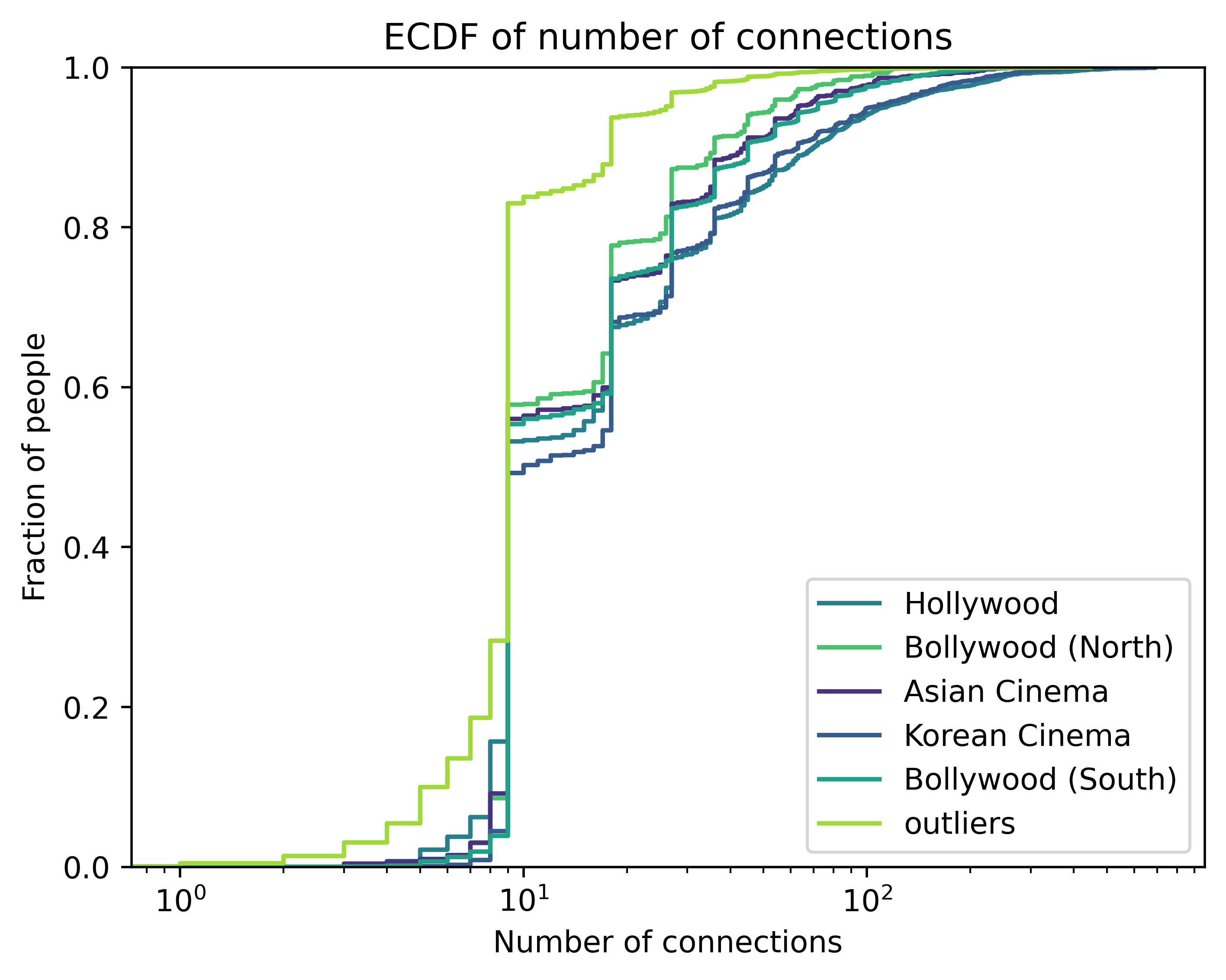
We see that connectivity is heavy-tailed. Additionally, outliers are less well-connected than any of the clusters. Interestingly, the distributions are very similar.
As the connectivity distribution is heavy-tailed, we consider the top 1% most connected outliers for our subsequent analysis. Indeed, it makes sense that outliers are less connected on average than cluster members. Otherwise they would have formed a cluster with other outliers or joined another cluster. For this reason, the most connected outliers are what is interesting. They are the ones that might be, for example, bridges between clusters. Equally well connected to both, which leads them not to be assigned to either of them.
But how well is this 1% connected to the others?
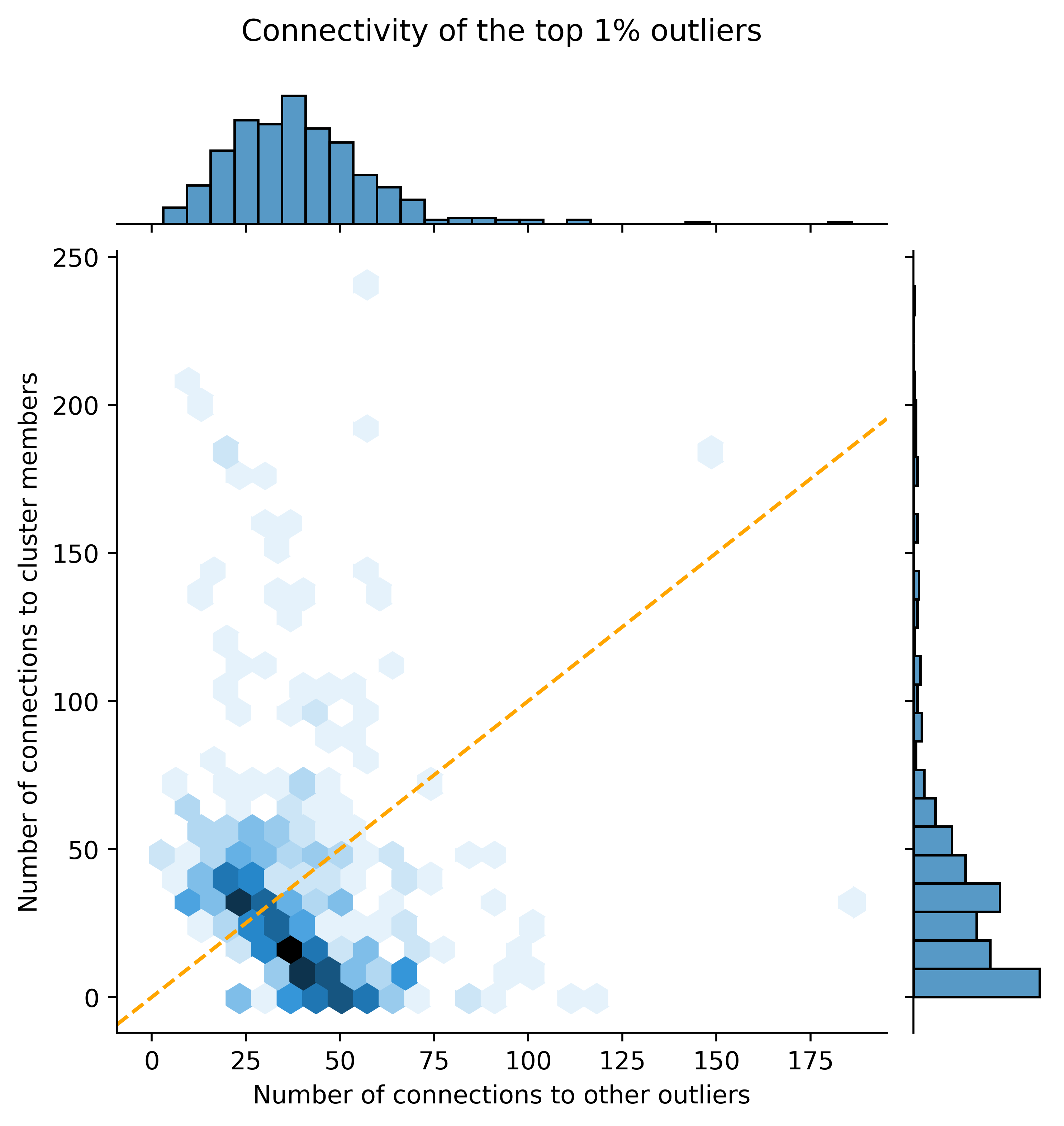
We see that even the top 1% of most connected outliers are not that well connected, with 74.7% having less than 100 connections. We see that some of them are truly isolated, but most of them are close to clusters.
Let’s look at who are these 1% outliers.
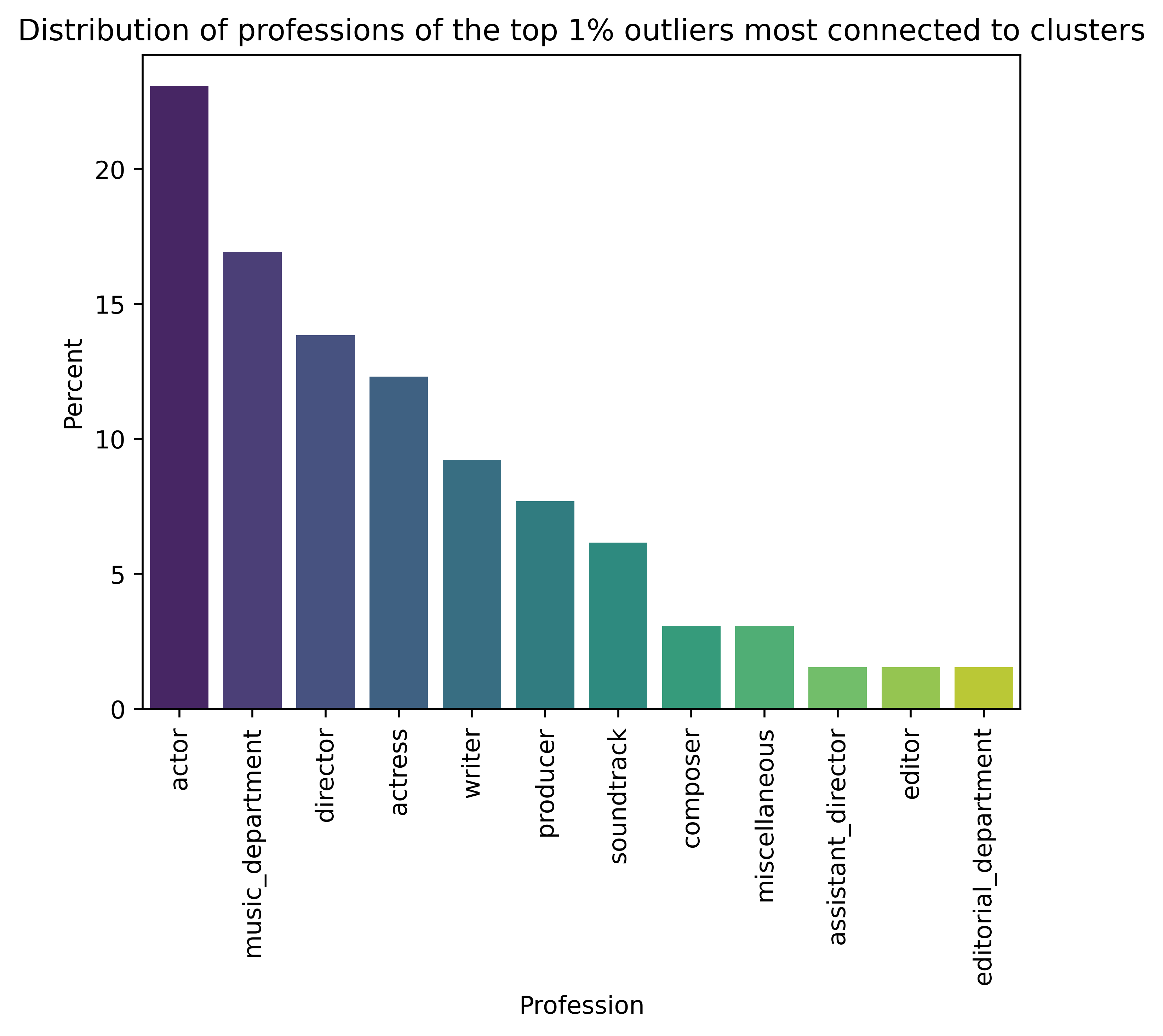
The plot shows that actors, music department directors and actresses are more likely to work globally. We can explain the lack of people with behind-the-scenes professions as outliers by saying that people with these professions are hired by film studios and they typically operate in their own countries.
Now let’s look at the ethnicity distribution of outliers. To compare, we also plotted the ethnicities of people with clusters.
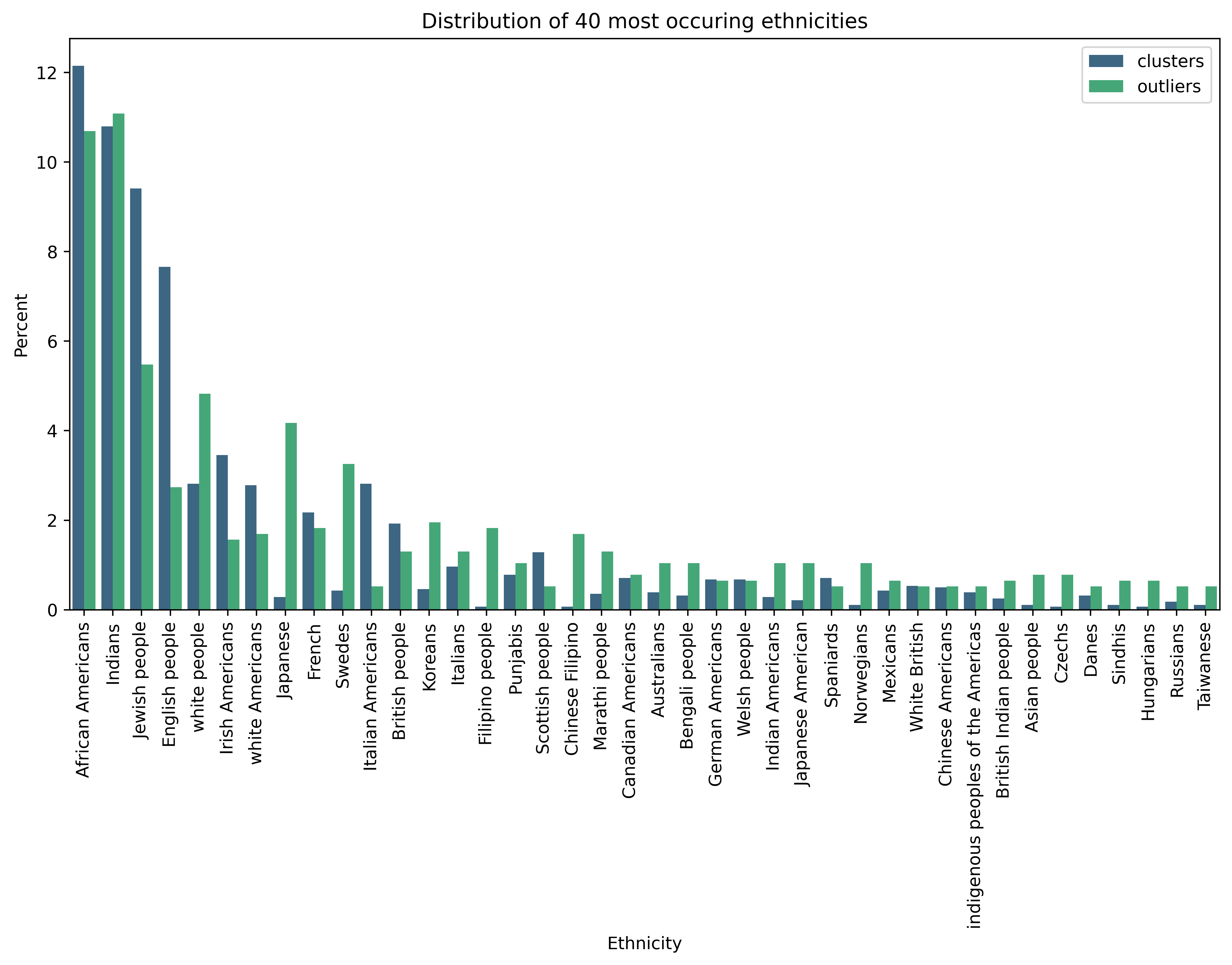
We observe that native English speakers are well represented in clusters, and they are also well represented in outliers. It makes sense since there are many movie industries that are located in English-speaking countries.
We see some ethnicities located in India and neighboring countries such as Punjabis, Marathis, Bengali and Sindhis who are outliers. This could indicate that their native movie industries are not big enough to be standalone. Hence their members often collaborate with people from other movie industry hotspots such as Bollywood.
Key People
We define the key people as outliers who have many connections to clusters or other outliers. Let’s look at two notable people.
- A.R. Rahman, an Indian music composer. He is mainly known in the West for his work on Slumdog Milionaire, for which he won 2 Oscars. He worked on 52 movies, almost exclusively from India. Due to his popularity there, he is very well connected to the two India related clusters (112 and 90 connections respectively), and to other outliers (225) connections, due to his involvement in music videos and tv series.

- Takashi Miike, a Japanese director most known for 13 Assassins. He directed 33 movies, and many more low-budget TV series. He has very little connection to clusters (5 connections to Hollywood cluster, 43 connections to Asian Cinema cluster) compared to his 250 connections to other outliers.
![]()
Conclusion
We used OPTICS clustering algorithm, a close relative to DBSCAN but allows rejecting clusters under a specific size which we chose as 400. When we looked at the common attributes of people in the same cluster, we saw that ethnicity value plays an important role. And we were able to map these clusters to real-life clusters. Some clusters had more people, and some had fewer due to the data we had. Merging the IMDb dataset with the CMU dataset allowed us to have more rich data. Since Freebase which CMU dataset was sourced from was built by volunteers, it had some biases towards the volunteers’ preferences, nationality and so on.
When we looked into the clusters, we saw that some clusters had more diverse ethnicities with non-negligible percentages. For example, Korean Cinema cluster was predominantly Korean (80%), whereas Hollwood had people from various ethnic backgrounds such as Jewish people and Italian Americans. Bollywood clusters also included many ethnic groups, which is not a surprise since India is very rich in ethnicities (74 listed in Wikipedia!).
In terms of genre preferences, drama leads everywhere. In the second place, Asian Cinema and Korean Cinema have action; Hollwood and Bollywood (North and South) have comedy.
When we were analyzing professions, we saw that there are fewer actresses than actors. Looking closer, we saw the gender gap which was very obvious in all clusters. While Korean Cinema was the “most” inclusive, Hollywood and Bollywood had an overwhelming majority of males. Ageism was also very present in Hollywood, and Korean Cinema has more representation of ages than others.
More than half of the people were outliers, so it was worth analyzing them. Some outliers had many connections to the people in clusters; some had more connections to other outliers or not many connections (loners in the industry).
Further Details
The primary dataset which was sourced from Freebase had many attribute values missing which led us to make further assumptions, however by using IMDb dataset which is more reliable, our assumptions hold.
Our results could vary depending on the clustering algorithm used, and the parameters we set, such as cluster size cutoff. For example, Jackie Chan, a famous Hong Kongese action comedy actor known globally, was placed in the Hollwood cluster. But he is at the very edge of the cluster (i.e. very close to being an outlier). He started his career in Hong Kong in 1962 when he was five years old. And he made his breakthrough in Hollywood in mid-1990s. He has played in 115 movies so far. He has been honored with The Hong Kong Star, in Hong Kong and a star on the Hollywood Walk of Fame. He is truly a key person in the movie industry.